Change Pivot Table Name
When you create a Pivot Table, Microsoft Excel automatically names the Pivot Table as PivotTable1 and the next Pivot Table that you create is named as PivotTable2. Instead of following this default naming convention, you can change Pivot Table Name to something meaningful and relevant to the data on the Pivot Table. For example, Pivot Tables with names “January Sales” or “Sales by Months” appear more meaningful, compared to default Excel generated names (PivotTable1 and PivotTable2) Another advantage of changing the default Names of Pivot Tables is that you will be able to reference them in formulas and in Visual basic coding.
Steps to Change Pivot Table Name
As mentioned above, it is really easy to change Pivot Table name in Microsoft Excel.
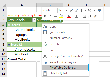
Right-click anywhere on the Pivot Table and then click on PivotTable Options… in the menu that appears.
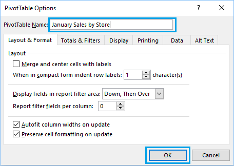
On Pivot Table Options screen, click in the box next to PivotTable Name and type the New Name for your Pivot Table. In our case, we have named our Pivot Table as “January Sales by Store”.
3. Once you are done, click on the OK button to save this change.
How to Add or Remove Subtotals in Pivot Table